Markus-Schirmer.com

Network theory is a growing area of interest in modern science and has found applications in many areas, such as social interactions, economics, flavours in recipes and gene-disease relations. Many people might have heard about the small-world phenomenon, or the "six degrees of separation". In 1969, Travers and Milgram found that a message can be passed on to any other person by relaying it through the social network of people. As an experiment they asked participants to pass a message to a person they did not know, by using their friends and friends of their friends, basically a human chain. They found that the message only had to travel past a small number of people (6 on average) in order to reach its destination.

But what exactly is a network? A simple way of understanding a network is by assuming that a set of objects are connected by some sort of link. The set of objects may represent, for example, human beings, products, ingredients, diseases or brain regions, whereas the links are relationships or structural connections. In mathematical terms each object is called a node in a graph or a network, where the links are referred to as edges.

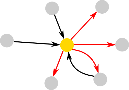
A graph or network can simply be represented by circles (nodes) and arrow (edges), where each edge can have a direction and weight. Directionality and weight can be understood in terms of friendship networks. Two people might see their relationship differently, in terms of how close they are or even if they are friends at all. Therefore a direction (who is friends with whom) and weight (strength of friendships) are useful information that can be incorporated in networks.

One of the simplest ways to characterise the nodes in a network is by their degree. The yellow node for example has 3 incoming edges and 4 outgoing edges, corresponding to an in- and out-degree of 3 and 4, respectively. Sometimes it can be useful to simplify a graph, for example by discarding the directionality information. In that case the yellow node would have a degree of 4. There are other measures that can be used to describe nodes or the complete network. The intuition behind some of the more popular ones are introduced in the network measures section. Other aspects can be quite important as well, such as a network's topology or how we can create random networks. All these principles can help us understand what happens in networks that are too large to deal with by just looking at them, as they can be found, for example, in the human brain, which connects 100 billion nodes (neurons) through 100 trillion edges (synapses).

We have already talked about the network measure degree. It is one of the simplest and most intuitive measures to describe individual nodes. This and many other nodal network measures can be used to describe entire networks as well. A common approach is to take the average over all nodes and use it as a representative measure of the network.

Clustering

The clustering coefficient is one of the most important network measures that has been used in a wide range of studies. It was first introduced in 1998 and represents the probability that two neighbours (connected by an edge) of a node are also connected, i.e. forming closed triangles. In social media it would represent the chance of a persons friends to be friends themselves. This way, the clustering coefficient can describe the extent of how cliquish friendship circles are.

The measure itself takes on values between 0 and 1, where a clustering coefficient of 1 is only achieved if the neighbourhood of a node is fully connected, i.e. that all of a person's friends are also friends with each other.

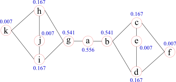
A similar measure, defined for the entire network however, is called transitivity. It is calculated over all the nodes and some consider it to be a more representative measure of the entire network, compared to the average clustering coefficient. An example where both measures can result in different trends when the network is slightly altered can be seen here:

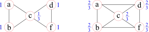
The network on the right is similar to the one on the left, with the exception that two more of all possible triangles in the network are formed. The average clustering coefficient (0.87→0.67), however, is reduced by closing these additional triangles, whereas transitivity (0.60→0.67) reflects this closing by an increase.

Modularity

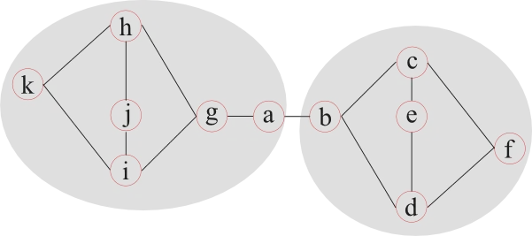
Modularity tries to determine how well a network can be separated into communities (modules). This is a challenging problem and many different approaches have been developed over the years. One possible approach splits a network into two parts and continues to split these subnetworks into smaller and smaller communities, as long as a measure of separation increases.

This example illustrates that the definition of two modules is not always well defined. Node a, for example, can belong to either module, while any measure of separation reaches equal values. Therefore most community finding algorithms are used multiple times on the same network and the average measure of separation can be used to describe the network.

Characteristic path-length and efficiency

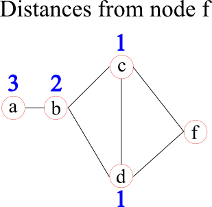
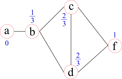
Some network measures are calculated on the shortest distances between nodes. In some cases, these can represent by physical distances, such as the distance between cities a person and his or her friend lives. However, sometimes these distances are unknown and/or the topological distances are of interest. Topological distances can be related, for example, to the weights (strenghts) of edges by using a function to map a weight into a distance or to the number of "hops" in binarised networks. In brain analyses, these distances are often set to the inverse edge weight. In the following graph the distances from node f to all other nodes are given by the blue numbers above each node.

Once these distances are defined, a network measure called characteristic path-length may be calculated. For each node it is given by the average distance to all other nodes (1.75 for node f in the example before). It represents how "central" a node is in the network.

A closely related network measure is called efficiency. Instead of taking the average of the distances, it uses the average over the inverse distances. The intuition behind this approach lies in the assumption that if two nodes are closer, the efficiency of their communication (information transport) is higher. Node f, for example, has an efficiency of 0.71. The benefit of efficiency over characteristic path-length lies in the meaningful calculation of the efficiency in networks that have two separate (unconnected) components. The efficiency of information transport between the two components is 0, whereas the characteristic path-length is infinity, which can cause "problems" when calculating a global network measure.

Betweenness centrality

Betweenness centrality provides a measure of a node's importance by counting how many of the shortest paths, not starting or ending at that particular node, pass through it. It was introduced by Freeman in 1977 and can be interpreted with respect to the information flow within a network.

When considering the flow of information or messages from node to node along the edges, betweenness centrality is a measure which relates to the amount of information passing through a certain node (assuming that information travels along the shortest paths). Betweenness centrality considers the load of a node, instead of how well it is connected. Therefore it can be seen as a measure of importance with respect to network functionality. It also means that a node with just two connections might have a high betweenness centrality in a network, for example, if it connects two communities of the network as in the previous figure.

There are many more measures than those described here. For a more detailed an mathematical discussion of the measures above, and references to other measures, please see a great overview by Rubinov and Sporns.

Network models are very important to understand organisational principles or to understand if an observed property of a network has occurred by chance or if there is something "special" about it. Over the years many different network models have been developed. We will talk briefly about the most important ones, where the importance is to be understood in their popularity in brain research or because they are "extremes" which are necessary to understand, for example in the context of network topology.

Ordered networks

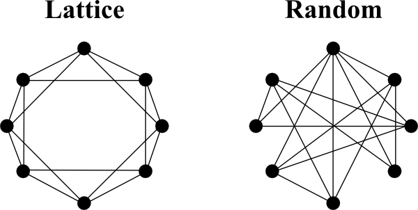
Ordered networks are commonly referred to as lattice networks. In these network models nodes are connected to their nearest neighbours, resulting in a large clustering coefficient. It represents one of the extreme ends of the network spectrum, which is uncommon in the real world, as information transport along the edges in the network takes relatively long. However, lattice networks are very resilient to attacks. If a particular node was knocked out, the overall network structure most likely would not suffer.

Lattice networks are sometimes referred to as geometric networks, as they may take the geometric positions of the nodes into account. This may be important, when networks are not only investigated in two dimensions, but in three, as they can be found for example in the brain. Visually representing large networks as above is challenging in three dimensions. In these cases it is common to represent a network with N nodes by their adjacency matrix - a matrix of size NxN filled with zeros and ones, depending if an edge between two nodes exist (one) or not (zero).

A circular lattice network, like the one above, can be represented by the adjacency matrix on the left (200x200 matrix, existing edges coloured in white). However, for example in brain network and when taking the geodesic distance (the distance along the surface) into account, the adjacency matrix is usually not that simple (matrix on the right).

Random networks

The ER graph is an easy way to generate a random network. However, unlike real networks, ER random graphs usually do not produce any hubs (nodes which have many more edges than the average in the graph). One interesting property, however, is the emergence of the giant component. Once the average nodal degree reaches one, a large amount of nodes become connected. In particular when considering information or disease transfer, the giant component allows for an extensive spread.

Other models include for example the preferential attachment model introduced by Barabási and colleagues. It is a dynamic network model, which means that it incorporates a time component. At each time step a new node is introduced into the network, which connects with one or more of the existing nodes depending on how long the nodes have been present in the network (the older the node, the higher the probability that a new node forms a connection with it). A good example of this kind network can be found when analysing the citations of scientific publications.

Surrogate networks

In order to assess if a given property is "special" in an observed network, it is important to compare it to a random realisation which shares some of its properties. These random networks can be seen as a baseline to which the observed network can be compared. Random realisations can be achieved for example by using the ER model as described before, and matching the number of nodes and number of edges. Another set of random graphs are the so-called exponential random graph models (ERGM). The user can specify any given parameter, such as values of a given network measure, and the ERGM then draw samples randomly from the set of all graphs that share this property. This approach, however, is computationally very expensive.

A very common method used to create surrogate networks in brain network analyses is based on the principle of pairwise switching. It randomises the edges of an observed graph, while keeping the degree of each node constant.

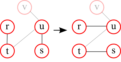
The principle is as follows: Two nodes in the graph are picked randomly (for example r and s). From the neighbourhood of each of these nodes (the nodes that are directly connected to them) a neighbour is selected randomly (for example t and u). In the next step the neighbours are exchanged. In the example above, this means that node s is connected to node t and node r to node u.

Different types of networks can show different types of network topology. Here we will briefly discuss the network topologies that can be found in many observed networks. Network models which can be used as surrogate networks are discussed in the network models section below.

Small-world

Almost 30 years after Travers and Milgram identified the small-world phenomenon, Watts and Strogatz described the underlying principles of small-world organisation in networks. They found that networks with a small-world organisation can be found between completely ordered networks (lattice) and completely random networks (Erdős-Rényi). A simple way of generating such a small-world topology is by randomly rewiring a small percentage of the edges of a lattice network, thereby creating "short-cuts" or long-range connections.

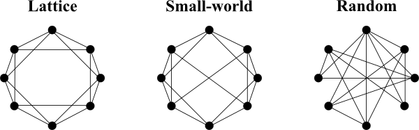
Networks with small-world topology therefore share properties of both lattice and random networks. Similar to lattice networks their clustering coefficient is high, however, compared to small-world networks, their characteristic path-length is small (similar to a random graph). Many real networks show these properties, making the small-world topology an important aspect when analysing graphs.

Rich-club

Another organisational principle focuses on the subnetwork consisting of nodes with a large percentage of connections within the network (so called hubs), which are densely inter-connected. Nodes belonging to the rich-club are rich in terms of a specified network metric, for example the number of edges. It can be said that the rich-club forms a backbone of the network and similar to internet backbones consists of principal routes between strategically interconnected nodes.

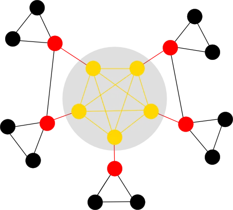
In the example above, the rich-club (and corresponding edges) are coloured in gold. The remainder of the network can then be classified into feeder (red) and local (black). The rich-club organisation has a variety of important implications, such as functional integration of nodes, resilience to random attacks and the possibility for nodal specialisation.